
Welcome to Course 5's first assignment! In this assignment, you will implement key components of a Recurrent Neural Network in numpy.
Recurrent Neural Networks (RNN) are very effective for Natural Language Processing and other sequence tasks because they have "memory". They can read inputs $x^{\langle t \rangle}$ (such as words) one at a time, and remember some information/context through the hidden layer activations that get passed from one time-step to the next. This allows a unidirectional RNN to take information from the past to process later inputs. A bidirectional RNN can take context from both the past and the future.
Notation:
Superscript $[l]$ denotes an object associated with the $l^{th}$ layer.
Superscript $(i)$ denotes an object associated with the $i^{th}$ example.
Superscript $\langle t \rangle$ denotes an object at the $t^{th}$ time-step.
Subscript $i$ denotes the $i^{th}$ entry of a vector.
Example:
numpy. #### START CODE HERE
#### END CODE HERE
# GRADED FUNCTION: routine_name
rnn_cell_backwardlstm_cell_backwardlstm_forwardlstm_cell_forwardLet's first import all the packages that you will need during this assignment.
import numpy as np
from rnn_utils import *
Later this week, you will generate music using an RNN. The basic RNN that you will implement has the structure below. In this example, $T_x = T_y$.
xt.a_prev or a_next, depending on the function that's being implemented.y_pred: $\hat{y}$ yt_pred: $\hat{y}^{\langle t \rangle}$Here's how you can implement an RNN:
Steps:
A recurrent neural network can be seen as the repeated use of a single cell. You are first going to implement the computations for a single time-step. The following figure describes the operations for a single time-step of an RNN cell.
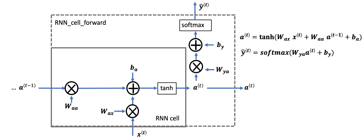
rnn_cell_forward, also calculates the prediction $\hat{y}^{\langle t \rangle}$Exercise: Implement the RNN-cell described in Figure (2).
Instructions:
softmax.cache.cachesoftmax function that you can use. It is located in the file 'rnn_utils.py' and has been imported.# GRADED FUNCTION: rnn_cell_forward
def rnn_cell_forward(xt, a_prev, parameters):
"""
Implements a single forward step of the RNN-cell as described in Figure (2)
Arguments:
xt -- your input data at timestep "t", numpy array of shape (n_x, m).
a_prev -- Hidden state at timestep "t-1", numpy array of shape (n_a, m)
parameters -- python dictionary containing:
Wax -- Weight matrix multiplying the input, numpy array of shape (n_a, n_x)
Waa -- Weight matrix multiplying the hidden state, numpy array of shape (n_a, n_a)
Wya -- Weight matrix relating the hidden-state to the output, numpy array of shape (n_y, n_a)
ba -- Bias, numpy array of shape (n_a, 1)
by -- Bias relating the hidden-state to the output, numpy array of shape (n_y, 1)
Returns:
a_next -- next hidden state, of shape (n_a, m)
yt_pred -- prediction at timestep "t", numpy array of shape (n_y, m)
cache -- tuple of values needed for the backward pass, contains (a_next, a_prev, xt, parameters)
"""
# Retrieve parameters from "parameters"
Wax = parameters["Wax"]
Waa = parameters["Waa"]
Wya = parameters["Wya"]
ba = parameters["ba"]
by = parameters["by"]
### START CODE HERE ### (≈2 lines)
# compute next activation state using the formula given above
a_next = np.tanh(np.dot(Waa, a_prev)+np.dot(Wax, xt) + ba)
# compute output of the current cell using the formula given above
yt_pred = softmax(np.dot(Wya, a_next)+by)
### END CODE HERE ###
# store values you need for backward propagation in cache
cache = (a_next, a_prev, xt, parameters)
return a_next, yt_pred, cache
np.random.seed(1)
xt_tmp = np.random.randn(3,10)
a_prev_tmp = np.random.randn(5,10)
parameters_tmp = {}
parameters_tmp['Waa'] = np.random.randn(5,5)
parameters_tmp['Wax'] = np.random.randn(5,3)
parameters_tmp['Wya'] = np.random.randn(2,5)
parameters_tmp['ba'] = np.random.randn(5,1)
parameters_tmp['by'] = np.random.randn(2,1)

a_next_tmp, yt_pred_tmp, cache_tmp = rnn_cell_forward(xt_tmp, a_prev_tmp, parameters_tmp)
print("a_next[4] = \n", a_next_tmp[4])
print("a_next.shape = \n", a_next_tmp.shape)
print("yt_pred[1] =\n", yt_pred_tmp[1])
print("yt_pred.shape = \n", yt_pred_tmp.shape)
a_next[4] =
 [ 0.59584544  0.18141802  0.61311866  0.99808218  0.85016201  0.99980978
 -0.18887155  0.99815551  0.6531151   0.82872037]
a_next.shape =
 (5, 10)
yt_pred[1] =
 [ 0.9888161   0.01682021  0.21140899  0.36817467  0.98988387  0.88945212
  0.36920224  0.9966312   0.9982559   0.17746526]
yt_pred.shape =
 (2, 10)
Expected Output:
a_next[4] =
 [ 0.59584544  0.18141802  0.61311866  0.99808218  0.85016201  0.99980978
 -0.18887155  0.99815551  0.6531151   0.82872037]
a_next.shape =
 (5, 10)
yt_pred[1] =
 [ 0.9888161   0.01682021  0.21140899  0.36817467  0.98988387  0.88945212
  0.36920224  0.9966312   0.9982559   0.17746526]
yt_pred.shape =
 (2, 10)
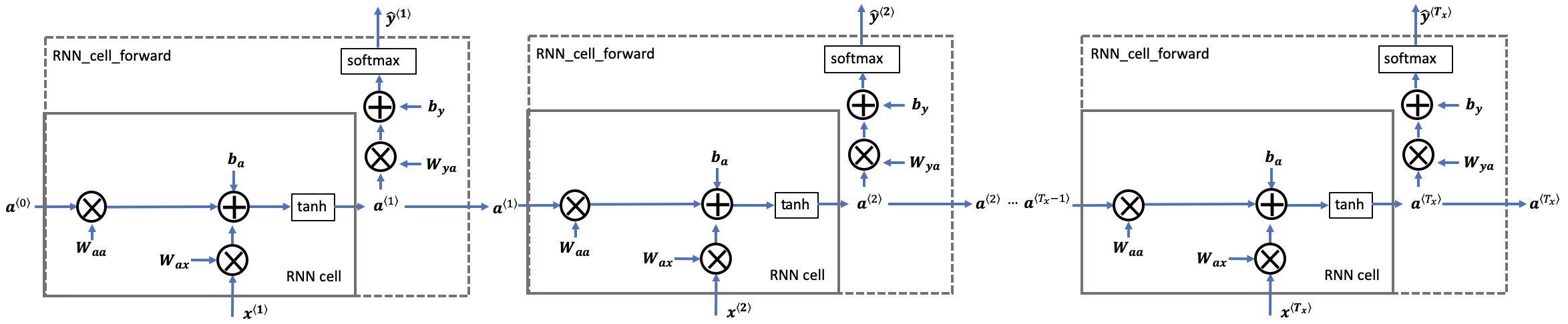
Exercise: Code the forward propagation of the RNN described in Figure (3).
Instructions:
a_next by setting it equal to the initial hidden state, $a_{0}$.a_next), the prediction $\hat{y}^{\langle t \rangle}$ and the cache by running rnn_cell_forward.yt_pred) in the 3D tensor $\hat{y}_{pred}$ at the $t^{th}$ position.var_name[:,:,i].# GRADED FUNCTION: rnn_forward
def rnn_forward(x, a0, parameters):
"""
Implement the forward propagation of the recurrent neural network described in Figure (3).
Arguments:
x -- Input data for every time-step, of shape (n_x, m, T_x).
a0 -- Initial hidden state, of shape (n_a, m)
parameters -- python dictionary containing:
Waa -- Weight matrix multiplying the hidden state, numpy array of shape (n_a, n_a)
Wax -- Weight matrix multiplying the input, numpy array of shape (n_a, n_x)
Wya -- Weight matrix relating the hidden-state to the output, numpy array of shape (n_y, n_a)
ba -- Bias numpy array of shape (n_a, 1)
by -- Bias relating the hidden-state to the output, numpy array of shape (n_y, 1)
Returns:
a -- Hidden states for every time-step, numpy array of shape (n_a, m, T_x)
y_pred -- Predictions for every time-step, numpy array of shape (n_y, m, T_x)
caches -- tuple of values needed for the backward pass, contains (list of caches, x)
"""
# Initialize "caches" which will contain the list of all caches
caches = []
# Retrieve dimensions from shapes of x and parameters["Wya"]
n_x, m, T_x = x.shape
n_y, n_a = parameters["Wya"].shape
### START CODE HERE ###
# initialize "a" and "y_pred" with zeros (≈2 lines)
a = np.zeros(shape=(n_a, m, T_x))
y_pred = np.zeros(shape=(n_y, m, T_x))
# Initialize a_next (≈1 line)
a_next = a0
# loop over all time-steps of the input 'x' (1 line)
for t in range(T_x):
# Update next hidden state, compute the prediction, get the cache (≈2 lines)
xt = x[:,:,t]
a_next, yt_pred, cache = rnn_cell_forward(xt, a_next, parameters)
# Save the value of the new "next" hidden state in a (≈1 line)
a[:,:,t] = a_next
# Save the value of the prediction in y (≈1 line)
y_pred[:,:,t] = yt_pred
# Append "cache" to "caches" (≈1 line)
caches.append(cache)
### END CODE HERE ###
# store values needed for backward propagation in cache
caches = (caches, x)
return a, y_pred, caches
np.random.seed(1)
x_tmp = np.random.randn(3,10,4)
a0_tmp = np.random.randn(5,10)
parameters_tmp = {}
parameters_tmp['Waa'] = np.random.randn(5,5)
parameters_tmp['Wax'] = np.random.randn(5,3)
parameters_tmp['Wya'] = np.random.randn(2,5)
parameters_tmp['ba'] = np.random.randn(5,1)
parameters_tmp['by'] = np.random.randn(2,1)

a_tmp, y_pred_tmp, caches_tmp = rnn_forward(x_tmp, a0_tmp, parameters_tmp)
print("a[4][1] = \n", a_tmp[4][1])
print("a.shape = \n", a_tmp.shape)
print("y_pred[1][3] =\n", y_pred_tmp[1][3])
print("y_pred.shape = \n", y_pred_tmp.shape)
print("caches[1][1][3] =\n", caches_tmp[1][1][3])
print("len(caches) = \n", len(caches_tmp))
a[4][1] =
 [-0.99999375  0.77911235 -0.99861469 -0.99833267]
a.shape =
 (5, 10, 4)
y_pred[1][3] =
 [ 0.79560373  0.86224861  0.11118257  0.81515947]
y_pred.shape =
 (2, 10, 4)
caches[1][1][3] =
 [-1.1425182  -0.34934272 -0.20889423  0.58662319]
len(caches) =
 2
Expected Output:
a[4][1] =
 [-0.99999375  0.77911235 -0.99861469 -0.99833267]
a.shape =
 (5, 10, 4)
y_pred[1][3] =
 [ 0.79560373  0.86224861  0.11118257  0.81515947]
y_pred.shape =
 (2, 10, 4)
caches[1][1][3] =
 [-1.1425182  -0.34934272 -0.20889423  0.58662319]
len(caches) =
 2
Congratulations! You've successfully built the forward propagation of a recurrent neural network from scratch.
In the next part, you will build a more complex LSTM model, which is better at addressing vanishing gradients. The LSTM will be better able to remember a piece of information and keep it saved for many timesteps.
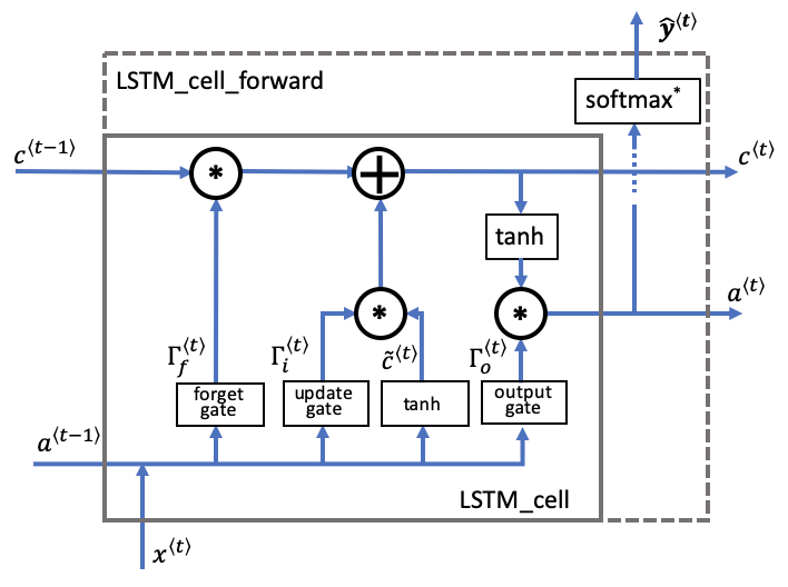
The following figure shows the operations of an LSTM-cell.
Similar to the RNN example above, you will start by implementing the LSTM cell for a single time-step. Then you can iteratively call it from inside a "for-loop" to have it process an input with $T_x$ time-steps.
The variable names in the code are similar to the equations, with slight differences.
Wf: forget gate weight $\mathbf{W}_{f}$bf: forget gate bias $\mathbf{b}_{f}$ft: forget gate $\Gamma_f^{\langle t \rangle}$cct: candidate value $\mathbf{\tilde{c}}^{\langle t \rangle}$In the code, we'll use the variable names found in the academic literature. These variables don't use "u" to denote "update".
Wi is the update gate weight $\mathbf{W}_i$ (not "Wu") bi is the update gate bias $\mathbf{b}_i$ (not "bu")it is the forget gate $\mathbf{\Gamma}_i^{\langle t \rangle}$ (not "ut")c: cell state, including all time steps, $\mathbf{c}$ shape $(n_{a}, m, T)$c_next: new (next) cell state, $\mathbf{c}^{\langle t \rangle}$ shape $(n_{a}, m)$c_prev: previous cell state, $\mathbf{c}^{\langle t-1 \rangle}$, shape $(n_{a}, m)$Wo: output gate weight, $\mathbf{W_o}$bo: output gate bias, $\mathbf{b_o}$ot: output gate, $\mathbf{\Gamma}_{o}^{\langle t \rangle}$a: hidden state, including time steps. $\mathbf{a}$ has shape $(n_{a}, m, T_{x})$a_next: hidden state for next time step. $\mathbf{a}^{\langle t \rangle}$ has shape $(n_{a}, m)$ The equation is: $$\mathbf{y}^{\langle t \rangle}_{pred} = \textrm{softmax}(\mathbf{W}_{y} \mathbf{a}^{\langle t \rangle} + \mathbf{b}_{y})$$
y_pred: prediction, including all time steps. $\mathbf{y}_{pred}$ has shape $(n_{y}, m, T_{x})$. Note that $(T_{y} = T_{x})$ for this example.yt_pred: prediction for the current time step $t$. $\mathbf{y}^{\langle t \rangle}_{pred}$ has shape $(n_{y}, m)$Exercise: Implement the LSTM cell described in the Figure (4).
Instructions:
axis parameter.sigmoid() and softmax are imported from rnn_utils.py.Wi, bi refer to the weights and biases of the update gate. There are no variables named "Wu" or "bu" in this function.# GRADED FUNCTION: lstm_cell_forward
def lstm_cell_forward(xt, a_prev, c_prev, parameters):
"""
Implement a single forward step of the LSTM-cell as described in Figure (4)
Arguments:
xt -- your input data at timestep "t", numpy array of shape (n_x, m).
a_prev -- Hidden state at timestep "t-1", numpy array of shape (n_a, m)
c_prev -- Memory state at timestep "t-1", numpy array of shape (n_a, m)
parameters -- python dictionary containing:
Wf -- Weight matrix of the forget gate, numpy array of shape (n_a, n_a + n_x)
bf -- Bias of the forget gate, numpy array of shape (n_a, 1)
Wi -- Weight matrix of the update gate, numpy array of shape (n_a, n_a + n_x)
bi -- Bias of the update gate, numpy array of shape (n_a, 1)
Wc -- Weight matrix of the first "tanh", numpy array of shape (n_a, n_a + n_x)
bc -- Bias of the first "tanh", numpy array of shape (n_a, 1)
Wo -- Weight matrix of the output gate, numpy array of shape (n_a, n_a + n_x)
bo -- Bias of the output gate, numpy array of shape (n_a, 1)
Wy -- Weight matrix relating the hidden-state to the output, numpy array of shape (n_y, n_a)
by -- Bias relating the hidden-state to the output, numpy array of shape (n_y, 1)
Returns:
a_next -- next hidden state, of shape (n_a, m)
c_next -- next memory state, of shape (n_a, m)
yt_pred -- prediction at timestep "t", numpy array of shape (n_y, m)
cache -- tuple of values needed for the backward pass, contains (a_next, c_next, a_prev, c_prev, xt, parameters)
Note: ft/it/ot stand for the forget/update/output gates, cct stands for the candidate value (c tilde),
c stands for the cell state (memory)
"""
# Retrieve parameters from "parameters"
Wf = parameters["Wf"] # forget gate weight
bf = parameters["bf"]
Wi = parameters["Wi"] # update gate weight (notice the variable name)
bi = parameters["bi"] # (notice the variable name)
Wc = parameters["Wc"] # candidate value weight
bc = parameters["bc"]
Wo = parameters["Wo"] # output gate weight
bo = parameters["bo"]
Wy = parameters["Wy"] # prediction weight
by = parameters["by"]
# Retrieve dimensions from shapes of xt and Wy
n_x, m = xt.shape
n_y, n_a = Wy.shape
### START CODE HERE ###
# Concatenate a_prev and xt (≈1 line)
concat = np.concatenate((a_prev, xt), axis=0) #axis=0 maane row borabor concat hobe
# Compute values for ft (forget gate), it (update gate),
# cct (candidate value), c_next (cell state),
# ot (output gate), a_next (hidden state) (≈6 lines)
ft = sigmoid(np.dot(Wf, concat) + bf) # forget gate Γ⟨t⟩f=σ(Wf[a⟨t−1⟩,x⟨t⟩]+bf)
it = sigmoid(np.dot(Wi, concat) + bi) # update gate Γ⟨t⟩i=σ(Wi[a⟨t−1⟩,x⟨t⟩]+bi)
cct = np.tanh(np.dot(Wc, concat) + bc) # candidate value c̃ ⟨t⟩=tanh(Wc[a⟨t−1⟩,x⟨t⟩]+bc)
c_next = ft*c_prev + it*cct # cell state c⟨t⟩=Γ⟨t⟩f∗c⟨t−1⟩+Γ⟨t⟩i∗c̃ ⟨t
ot = sigmoid(np.dot(Wo, concat) + bo) # output gate Γ⟨t⟩o=σ(Wo[a⟨t−1⟩,x⟨t⟩]+bo)
a_next = ot*np.tanh(c_next) # hidden state a⟨t⟩=Γ⟨t⟩o∗tanh(c⟨t⟩)
# Compute prediction of the LSTM cell (≈1 line)
yt_pred = softmax(np.dot(Wy, a_next) + by) # y⟨t⟩pred=softmax(Wya⟨t⟩+by)
### END CODE HERE ###
# store values needed for backward propagation in cache
cache = (a_next, c_next, a_prev, c_prev, ft, it, cct, ot, xt, parameters)
return a_next, c_next, yt_pred, cache
np.random.seed(1)
xt_tmp = np.random.randn(3,10)
a_prev_tmp = np.random.randn(5,10)
c_prev_tmp = np.random.randn(5,10)
parameters_tmp = {}
parameters_tmp['Wf'] = np.random.randn(5, 5+3)
parameters_tmp['bf'] = np.random.randn(5,1)
parameters_tmp['Wi'] = np.random.randn(5, 5+3)
parameters_tmp['bi'] = np.random.randn(5,1)
parameters_tmp['Wo'] = np.random.randn(5, 5+3)
parameters_tmp['bo'] = np.random.randn(5,1)
parameters_tmp['Wc'] = np.random.randn(5, 5+3)
parameters_tmp['bc'] = np.random.randn(5,1)
parameters_tmp['Wy'] = np.random.randn(2,5)
parameters_tmp['by'] = np.random.randn(2,1)

a_next_tmp, c_next_tmp, yt_tmp, cache_tmp = lstm_cell_forward(xt_tmp, a_prev_tmp, c_prev_tmp, parameters_tmp)
print("a_next[4] = \n", a_next_tmp[4])
print("a_next.shape = ", a_next_tmp.shape)
print("c_next[2] = \n", c_next_tmp[2])
print("c_next.shape = ", c_next_tmp.shape)
print("yt[1] =", yt_tmp[1])
print("yt.shape = ", yt_tmp.shape)
print("cache[1][3] =\n", cache_tmp[1][3])
print("len(cache) = ", len(cache_tmp))
a_next[4] =
 [-0.66408471  0.0036921   0.02088357  0.22834167 -0.85575339  0.00138482
  0.76566531  0.34631421 -0.00215674  0.43827275]
a_next.shape =  (5, 10)
c_next[2] =
 [ 0.63267805  1.00570849  0.35504474  0.20690913 -1.64566718  0.11832942
  0.76449811 -0.0981561  -0.74348425 -0.26810932]
c_next.shape =  (5, 10)
yt[1] = [ 0.79913913  0.15986619  0.22412122  0.15606108  0.97057211  0.31146381
  0.00943007  0.12666353  0.39380172  0.07828381]
yt.shape =  (2, 10)
cache[1][3] =
 [-0.16263996  1.03729328  0.72938082 -0.54101719  0.02752074 -0.30821874
  0.07651101 -1.03752894  1.41219977 -0.37647422]
len(cache) =  10
Expected Output:
a_next[4] =
 [-0.66408471  0.0036921   0.02088357  0.22834167 -0.85575339  0.00138482
  0.76566531  0.34631421 -0.00215674  0.43827275]
a_next.shape =  (5, 10)
c_next[2] =
 [ 0.63267805  1.00570849  0.35504474  0.20690913 -1.64566718  0.11832942
  0.76449811 -0.0981561  -0.74348425 -0.26810932]
c_next.shape =  (5, 10)
yt[1] = [ 0.79913913  0.15986619  0.22412122  0.15606108  0.97057211  0.31146381
  0.00943007  0.12666353  0.39380172  0.07828381]
yt.shape =  (2, 10)
cache[1][3] =
 [-0.16263996  1.03729328  0.72938082 -0.54101719  0.02752074 -0.30821874
  0.07651101 -1.03752894  1.41219977 -0.37647422]
len(cache) =  10
Now that you have implemented one step of an LSTM, you can now iterate this over this using a for-loop to process a sequence of $T_x$ inputs.
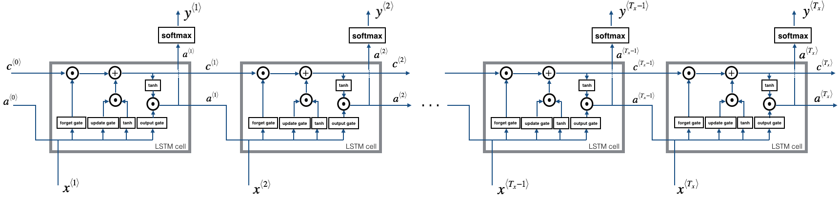
Exercise: Implement lstm_forward() to run an LSTM over $T_x$ time-steps.
Instructions
x and parameters.a_next.a0.c_next. c_next as its own variable with its own location in memory. Do not initialize it as a slice of the 3D tensor $c$. In other words, don't do c_next = c[:,:,0].lstm_cell_forward function that you defined previously, to get the hidden state, cell state, prediction, and cache.# GRADED FUNCTION: lstm_forward
def lstm_forward(x, a0, parameters):
"""
Implement the forward propagation of the recurrent neural network using an LSTM-cell described in Figure (4).
Arguments:
x -- Input data for every time-step, of shape (n_x, m, T_x).
a0 -- Initial hidden state, of shape (n_a, m)
parameters -- python dictionary containing:
Wf -- Weight matrix of the forget gate, numpy array of shape (n_a, n_a + n_x)
bf -- Bias of the forget gate, numpy array of shape (n_a, 1)
Wi -- Weight matrix of the update gate, numpy array of shape (n_a, n_a + n_x)
bi -- Bias of the update gate, numpy array of shape (n_a, 1)
Wc -- Weight matrix of the first "tanh", numpy array of shape (n_a, n_a + n_x)
bc -- Bias of the first "tanh", numpy array of shape (n_a, 1)
Wo -- Weight matrix of the output gate, numpy array of shape (n_a, n_a + n_x)
bo -- Bias of the output gate, numpy array of shape (n_a, 1)
Wy -- Weight matrix relating the hidden-state to the output, numpy array of shape (n_y, n_a)
by -- Bias relating the hidden-state to the output, numpy array of shape (n_y, 1)
Returns:
a -- Hidden states for every time-step, numpy array of shape (n_a, m, T_x)
y -- Predictions for every time-step, numpy array of shape (n_y, m, T_x)
c -- The value of the cell state, numpy array of shape (n_a, m, T_x)
caches -- tuple of values needed for the backward pass, contains (list of all the caches, x)
"""
# Initialize "caches", which will track the list of all the caches
caches = []
### START CODE HERE ###
Wy = parameters['Wy'] # saving parameters['Wy'] in a local variable in case students use Wy instead of parameters['Wy']
# Retrieve dimensions from shapes of x and parameters['Wy'] (≈2 lines)
n_x, m, T_x = x.shape
n_y, n_a = parameters['Wy'].shape
# initialize "a", "c" and "y" with zeros (≈3 lines)
a = np.zeros(shape=(n_a, m, T_x))
c = np.zeros_like(a) # c = a kora jabena. reference er jonno problem korte pare
y = np.zeros(shape=(n_y, m, T_x))
# Initialize a_next and c_next (≈2 lines)
a_next = a0
c_next = np.zeros_like(a_next) # c = a kora jabena. reference er jonno problem korte pare
# loop over all time-steps
for t in range(T_x):
# Get the 2D slice 'xt' from the 3D input 'x' at time step 't'
xt = x[:,:,t]
# Update next hidden state, next memory state, compute the prediction, get the cache (≈1 line)
a_next, c_next, yt, cache = lstm_cell_forward(xt, a_next, c_next, parameters)
# Save the value of the new "next" hidden state in a (≈1 line)
a[:,:,t] = a_next
# Save the value of the next cell state (≈1 line)
c[:,:,t] = c_next
# Save the value of the prediction in y (≈1 line)
y[:,:,t] = yt
# Append the cache into caches (≈1 line)
caches.append(cache)
### END CODE HERE ###
# store values needed for backward propagation in cache
caches = (caches, x)
return a, y, c, caches
np.random.seed(1)
x_tmp = np.random.randn(3,10,7)
a0_tmp = np.random.randn(5,10)
parameters_tmp = {}
parameters_tmp['Wf'] = np.random.randn(5, 5+3)
parameters_tmp['bf'] = np.random.randn(5,1)
parameters_tmp['Wi'] = np.random.randn(5, 5+3)
parameters_tmp['bi']= np.random.randn(5,1)
parameters_tmp['Wo'] = np.random.randn(5, 5+3)
parameters_tmp['bo'] = np.random.randn(5,1)
parameters_tmp['Wc'] = np.random.randn(5, 5+3)
parameters_tmp['bc'] = np.random.randn(5,1)
parameters_tmp['Wy'] = np.random.randn(2,5)
parameters_tmp['by'] = np.random.randn(2,1)

a_tmp, y_tmp, c_tmp, caches_tmp = lstm_forward(x_tmp, a0_tmp, parameters_tmp)
print("a[4][3][6] = ", a_tmp[4][3][6])
print("a.shape = ", a_tmp.shape)
print("y[1][4][3] =", y_tmp[1][4][3])
print("y.shape = ", y_tmp.shape)
print("caches[1][1][1] =\n", caches_tmp[1][1][1])
print("c[1][2][1]", c_tmp[1][2][1])
print("len(caches) = ", len(caches_tmp))
a[4][3][6] =  0.172117767533
a.shape =  (5, 10, 7)
y[1][4][3] = 0.95087346185
y.shape =  (2, 10, 7)
caches[1][1][1] =
 [ 0.82797464  0.23009474  0.76201118 -0.22232814 -0.20075807  0.18656139
  0.41005165]
c[1][2][1] -0.855544916718
len(caches) =  2
Expected Output:
a[4][3][6] =  0.172117767533
a.shape =  (5, 10, 7)
y[1][4][3] = 0.95087346185
y.shape =  (2, 10, 7)
caches[1][1][1] =
 [ 0.82797464  0.23009474  0.76201118 -0.22232814 -0.20075807  0.18656139
  0.41005165]
c[1][2][1] -0.855544916718
len(caches) =  2
Congratulations! You have now implemented the forward passes for the basic RNN and the LSTM. When using a deep learning framework, implementing the forward pass is sufficient to build systems that achieve great performance.
The rest of this notebook is optional, and will not be graded.
In modern deep learning frameworks, you only have to implement the forward pass, and the framework takes care of the backward pass, so most deep learning engineers do not need to bother with the details of the backward pass. If however you are an expert in calculus and want to see the details of backprop in RNNs, you can work through this optional portion of the notebook.
When in an earlier course you implemented a simple (fully connected) neural network, you used backpropagation to compute the derivatives with respect to the cost to update the parameters. Similarly, in recurrent neural networks you can calculate the derivatives with respect to the cost in order to update the parameters. The backprop equations are quite complicated and we did not derive them in lecture. However, we will briefly present them below.
Note that this notebook does not implement the backward path from the Loss 'J' backwards to 'a'. This would have included the dense layer and softmax which are a part of the forward path. This is assumed to be calculated elsewhere and the result passed to rnn_backward in 'da'. It is further assumed that loss has been adjusted for batch size (m) and division by the number of examples is not required here.
This section is optional and ungraded. It is more difficult and has fewer details regarding its implementation. This section only implements key elements of the full path.
We will start by computing the backward pass for the basic RNN-cell and then in the following sections, iterate through the cells.

Recall from lecture, the shorthand for the partial derivative of cost relative to a variable is dVariable. For example, $\frac{\partial J}{\partial W_{ax}}$ is $dW_{ax}$. This will be used throughout the remaining sections.

To compute the rnn_cell_backward you can utilize the following equations. It is a good exercise to derive them by hand. Here, $*$ denotes element-wise multiplication while the absence of a symbol indicates matrix multiplication.
\begin{align} \displaystyle a^{\langle t \rangle} &= \tanh(W_{ax} x^{\langle t \rangle} + W_{aa} a^{\langle t-1 \rangle} + b_{a})\tag{-} \\[8pt] \displaystyle \frac{\partial \tanh(x)} {\partial x} &= 1 - \tanh^2(x) \tag{-} \\[8pt] \displaystyle {dW_{ax}} &= (da_{next} * ( 1-\tanh^2(W_{ax}x^{\langle t \rangle}+W_{aa} a^{\langle t-1 \rangle} + b_{a}) )) x^{\langle t \rangle T}\tag{1} \\[8pt] \displaystyle dW_{aa} &= (da_{next} * ( 1-\tanh^2(W_{ax}x^{\langle t \rangle}+W_{aa} a^{\langle t-1 \rangle} + b_{a}) )) a^{\langle t-1 \rangle T}\tag{2} \\[8pt] \displaystyle db_a& = \sum_{batch}( da_{next} * ( 1-\tanh^2(W_{ax}x^{\langle t \rangle}+W_{aa} a^{\langle t-1 \rangle} + b_{a}) ))\tag{3} \\[8pt] \displaystyle dx^{\langle t \rangle} &= { W_{ax}}^T (da_{next} * ( 1-\tanh^2(W_{ax}x^{\langle t \rangle}+W_{aa} a^{\langle t-1 \rangle} + b_{a}) ))\tag{4} \\[8pt] \displaystyle da_{prev} &= { W_{aa}}^T(da_{next} * ( 1-\tanh^2(W_{ax}x^{\langle t \rangle}+W_{aa} a^{\langle t-1 \rangle} + b_{a}) ))\tag{5} \end{align}The results can be computed directly by implementing the equations above. However, the above can optionally be simplified by computing 'dz' and utlilizing the chain rule.
This can be further simplified by noting that $\tanh(W_{ax}x^{\langle t \rangle}+W_{aa} a^{\langle t-1 \rangle} + b_{a})$ was computed and saved in the forward pass.
To calculate dba, the 'batch' above is a sum across all 'm' examples (axis= 1). Note that you should use the keepdims = True option.
It may be worthwhile to review Course 1 Derivatives with a computational graph through Backpropagation Intuition, which decompose the calculation into steps using the chain rule.
Matrix vector derivatives are described here, though the equations above incorporate the required transformations.
Note rnn_cell_backward does not include the calculation of loss from $y \langle t \rangle$, this is incorporated into the incoming da_next. This is a slight mismatch with rnn_cell_forward which includes a dense layer and softmax.
Note: in the code:
$\displaystyle dx^{\langle t \rangle}$ is represented by dxt,
$\displaystyle d W_{ax}$ is represented by dWax,
$\displaystyle da_{prev}$ is represented by daprev,
$\displaystyle dW{aa}$ is represented by dWaa,
$\displaystyle db_{a}$ is represented by dba,
dz is not derived above but can optionally be derived by students to simplify the repeated calculations.
def rnn_cell_backward(da_next, cache):
    """
    Implements the backward pass for the RNN-cell (single time-step).

    Arguments:
    da_next -- Gradient of loss with respect to next hidden state
    cache -- python dictionary containing useful values (output of rnn_cell_forward())

    Returns:
    gradients -- python dictionary containing:
                        dx -- Gradients of input data, of shape (n_x, m)
                        da_prev -- Gradients of previous hidden state, of shape (n_a, m)
                        dWax -- Gradients of input-to-hidden weights, of shape (n_a, n_x)
                        dWaa -- Gradients of hidden-to-hidden weights, of shape (n_a, n_a)
                        dba -- Gradients of bias vector, of shape (n_a, 1)
    """

    # Retrieve values from cache
    (a_next, a_prev, xt, parameters) = cache

    # Retrieve values from parameters
    Wax = parameters["Wax"]
    Waa = parameters["Waa"]
    Wya = parameters["Wya"]
    ba = parameters["ba"]
    by = parameters["by"]

    ### START CODE HERE ###
    # compute the gradient of the loss with respect to z (optional) (≈1 line)
    dz = None

    # compute the gradient of the loss with respect to Wax (≈2 lines)
    dxt = None
    dWax = None

    # compute the gradient with respect to Waa (≈2 lines)
    da_prev = None
    dWaa = None

    # compute the gradient with respect to b (≈1 line)
    dba = None

    ### END CODE HERE ###

    # Store the gradients in a python dictionary
    gradients = {"dxt": dxt, "da_prev": da_prev, "dWax": dWax, "dWaa": dWaa, "dba": dba}

    return gradients
np.random.seed(1)
xt_tmp = np.random.randn(3,10)
a_prev_tmp = np.random.randn(5,10)
parameters_tmp = {}
parameters_tmp['Wax'] = np.random.randn(5,3)
parameters_tmp['Waa'] = np.random.randn(5,5)
parameters_tmp['Wya'] = np.random.randn(2,5)
parameters_tmp['ba'] = np.random.randn(5,1)
parameters_tmp['by'] = np.random.randn(2,1)

a_next_tmp, yt_tmp, cache_tmp = rnn_cell_forward(xt_tmp, a_prev_tmp, parameters_tmp)

da_next_tmp = np.random.randn(5,10)
gradients_tmp = rnn_cell_backward(da_next_tmp, cache_tmp)
print("gradients[\"dxt\"][1][2] =", gradients_tmp["dxt"][1][2])
print("gradients[\"dxt\"].shape =", gradients_tmp["dxt"].shape)
print("gradients[\"da_prev\"][2][3] =", gradients_tmp["da_prev"][2][3])
print("gradients[\"da_prev\"].shape =", gradients_tmp["da_prev"].shape)
print("gradients[\"dWax\"][3][1] =", gradients_tmp["dWax"][3][1])
print("gradients[\"dWax\"].shape =", gradients_tmp["dWax"].shape)
print("gradients[\"dWaa\"][1][2] =", gradients_tmp["dWaa"][1][2])
print("gradients[\"dWaa\"].shape =", gradients_tmp["dWaa"].shape)
print("gradients[\"dba\"][4] =", gradients_tmp["dba"][4])
print("gradients[\"dba\"].shape =", gradients_tmp["dba"].shape)
Expected Output:
| **gradients["dxt"][1][2]** = | -1.3872130506 |
| **gradients["dxt"].shape** = | (3, 10) |
| **gradients["da_prev"][2][3]** = | -0.152399493774 |
| **gradients["da_prev"].shape** = | (5, 10) |
| **gradients["dWax"][3][1]** = | 0.410772824935 |
| **gradients["dWax"].shape** = | (5, 3) |
| **gradients["dWaa"][1][2]** = | 1.15034506685 |
| **gradients["dWaa"].shape** = | (5, 5) |
| **gradients["dba"][4]** = | [ 0.20023491] |
| **gradients["dba"].shape** = | (5, 1) |
Computing the gradients of the cost with respect to $a^{\langle t \rangle}$ at every time-step $t$ is useful because it is what helps the gradient backpropagate to the previous RNN-cell. To do so, you need to iterate through all the time steps starting at the end, and at each step, you increment the overall $db_a$, $dW_{aa}$, $dW_{ax}$ and you store $dx$.
Instructions:
Implement the rnn_backward function. Initialize the return variables with zeros first and then loop through all the time steps while calling the rnn_cell_backward at each time timestep, update the other variables accordingly.
def rnn_backward(da, caches):
    """
    Implement the backward pass for a RNN over an entire sequence of input data.

    Arguments:
    da -- Upstream gradients of all hidden states, of shape (n_a, m, T_x)
    caches -- tuple containing information from the forward pass (rnn_forward)

    Returns:
    gradients -- python dictionary containing:
                        dx -- Gradient w.r.t. the input data, numpy-array of shape (n_x, m, T_x)
                        da0 -- Gradient w.r.t the initial hidden state, numpy-array of shape (n_a, m)
                        dWax -- Gradient w.r.t the input's weight matrix, numpy-array of shape (n_a, n_x)
                        dWaa -- Gradient w.r.t the hidden state's weight matrix, numpy-arrayof shape (n_a, n_a)
                        dba -- Gradient w.r.t the bias, of shape (n_a, 1)
    """

    ### START CODE HERE ###

    # Retrieve values from the first cache (t=1) of caches (≈2 lines)
    (caches, x) = None
    (a1, a0, x1, parameters) = None

    # Retrieve dimensions from da's and x1's shapes (≈2 lines)
    n_a, m, T_x = None
    n_x, m = None

    # initialize the gradients with the right sizes (≈6 lines)
    dx = None
    dWax = None
    dWaa = None
    dba = None
    da0 = None
    da_prevt = None

    # Loop through all the time steps
    for t in reversed(range(None)):
        # Compute gradients at time step t.
        # Remember to sum gradients from the output path (da) and the previous timesteps (da_prevt) (≈1 line)
        gradients = None
        # Retrieve derivatives from gradients (≈ 1 line)
        dxt, da_prevt, dWaxt, dWaat, dbat = gradients["dxt"], gradients["da_prev"], gradients["dWax"], gradients["dWaa"], gradients["dba"]
        # Increment global derivatives w.r.t parameters by adding their derivative at time-step t (≈4 lines)
        dx[:, :, t] = None
        dWax += None
        dWaa += None
        dba += None

    # Set da0 to the gradient of a which has been backpropagated through all time-steps (≈1 line)
    da0 = None
    ### END CODE HERE ###

    # Store the gradients in a python dictionary
    gradients = {"dx": dx, "da0": da0, "dWax": dWax, "dWaa": dWaa,"dba": dba}

    return gradients
np.random.seed(1)
x_tmp = np.random.randn(3,10,4)
a0_tmp = np.random.randn(5,10)
parameters_tmp = {}
parameters_tmp['Wax'] = np.random.randn(5,3)
parameters_tmp['Waa'] = np.random.randn(5,5)
parameters_tmp['Wya'] = np.random.randn(2,5)
parameters_tmp['ba'] = np.random.randn(5,1)
parameters_tmp['by'] = np.random.randn(2,1)

a_tmp, y_tmp, caches_tmp = rnn_forward(x_tmp, a0_tmp, parameters_tmp)
da_tmp = np.random.randn(5, 10, 4)
gradients_tmp = rnn_backward(da_tmp, caches_tmp)

print("gradients[\"dx\"][1][2] =", gradients_tmp["dx"][1][2])
print("gradients[\"dx\"].shape =", gradients_tmp["dx"].shape)
print("gradients[\"da0\"][2][3] =", gradients_tmp["da0"][2][3])
print("gradients[\"da0\"].shape =", gradients_tmp["da0"].shape)
print("gradients[\"dWax\"][3][1] =", gradients_tmp["dWax"][3][1])
print("gradients[\"dWax\"].shape =", gradients_tmp["dWax"].shape)
print("gradients[\"dWaa\"][1][2] =", gradients_tmp["dWaa"][1][2])
print("gradients[\"dWaa\"].shape =", gradients_tmp["dWaa"].shape)
print("gradients[\"dba\"][4] =", gradients_tmp["dba"][4])
print("gradients[\"dba\"].shape =", gradients_tmp["dba"].shape)
Expected Output:
| **gradients["dx"][1][2]** = | [-2.07101689 -0.59255627 0.02466855 0.01483317] |
| **gradients["dx"].shape** = | (3, 10, 4) |
| **gradients["da0"][2][3]** = | -0.314942375127 |
| **gradients["da0"].shape** = | (5, 10) |
| **gradients["dWax"][3][1]** = | 11.2641044965 |
| **gradients["dWax"].shape** = | (5, 3) |
| **gradients["dWaa"][1][2]** = | 2.30333312658 |
| **gradients["dWaa"].shape** = | (5, 5) |
| **gradients["dba"][4]** = | [-0.74747722] |
| **gradients["dba"].shape** = | (5, 1) |
The LSTM backward pass is slightly more complicated than the forward pass.

The equations for the LSTM backward pass are provided below. (If you enjoy calculus exercises feel free to try deriving these from scratch yourself.)
Note the location of the gate derivatives ($\gamma$..) between the dense layer and the activation function (see graphic above). This is convenient for computing parameter derivatives in the next step. \begin{align} d\gamma_o^{\langle t \rangle} &= da_{next}*\tanh(c_{next}) * \Gamma_o^{\langle t \rangle}*\left(1-\Gamma_o^{\langle t \rangle}\right)\tag{7} \\[8pt] dp\widetilde{c}^{\langle t \rangle} &= \left(dc_{next}*\Gamma_u^{\langle t \rangle}+ \Gamma_o^{\langle t \rangle}* (1-\tanh^2(c_{next})) * \Gamma_u^{\langle t \rangle} * da_{next} \right) * \left(1-\left(\widetilde c^{\langle t \rangle}\right)^2\right) \tag{8} \\[8pt] d\gamma_u^{\langle t \rangle} &= \left(dc_{next}*\widetilde{c}^{\langle t \rangle} + \Gamma_o^{\langle t \rangle}* (1-\tanh^2(c_{next})) * \widetilde{c}^{\langle t \rangle} * da_{next}\right)*\Gamma_u^{\langle t \rangle}*\left(1-\Gamma_u^{\langle t \rangle}\right)\tag{9} \\[8pt] d\gamma_f^{\langle t \rangle} &= \left(dc_{next}* c_{prev} + \Gamma_o^{\langle t \rangle} * (1-\tanh^2(c_{next})) * c_{prev} * da_{next}\right)*\Gamma_f^{\langle t \rangle}*\left(1-\Gamma_f^{\langle t \rangle}\right)\tag{10} \end{align}
$ dW_f = d\gamma_f^{\langle t \rangle} \begin{bmatrix} a_{prev} \\ x_t\end{bmatrix}^T \tag{11} $ $ dW_u = d\gamma_u^{\langle t \rangle} \begin{bmatrix} a_{prev} \\ x_t\end{bmatrix}^T \tag{12} $ $ dW_c = dp\widetilde c^{\langle t \rangle} \begin{bmatrix} a_{prev} \\ x_t\end{bmatrix}^T \tag{13} $ $ dW_o = d\gamma_o^{\langle t \rangle} \begin{bmatrix} a_{prev} \\ x_t\end{bmatrix}^T \tag{14}$
To calculate $db_f, db_u, db_c, db_o$ you just need to sum across all 'm' examples (axis= 1) on $d\gamma_f^{\langle t \rangle}, d\gamma_u^{\langle t \rangle}, dp\widetilde c^{\langle t \rangle}, d\gamma_o^{\langle t \rangle}$ respectively. Note that you should have the keepdims = True option.
$\displaystyle db_f = \sum_{batch}d\gamma_f^{\langle t \rangle}\tag{15}$ $\displaystyle db_u = \sum_{batch}d\gamma_u^{\langle t \rangle}\tag{16}$ $\displaystyle db_c = \sum_{batch}d\gamma_c^{\langle t \rangle}\tag{17}$ $\displaystyle db_o = \sum_{batch}d\gamma_o^{\langle t \rangle}\tag{18}$
Finally, you will compute the derivative with respect to the previous hidden state, previous memory state, and input.
$ da_{prev} = W_f^T d\gamma_f^{\langle t \rangle} + W_u^T d\gamma_u^{\langle t \rangle}+ W_c^T dp\widetilde c^{\langle t \rangle} + W_o^T d\gamma_o^{\langle t \rangle} \tag{19}$
Here, to account for concatenation, the weights for equations 19 are the first n_a, (i.e. $W_f = W_f[:,:n_a]$ etc...)
$ dc_{prev} = dc_{next}*\Gamma_f^{\langle t \rangle} + \Gamma_o^{\langle t \rangle} * (1- \tanh^2(c_{next}))*\Gamma_f^{\langle t \rangle}*da_{next} \tag{20}$
$ dx^{\langle t \rangle} = W_f^T d\gamma_f^{\langle t \rangle} + W_u^T d\gamma_u^{\langle t \rangle}+ W_c^T dp\widetilde c^{\langle t \rangle} + W_o^T d\gamma_o^{\langle t \rangle}\tag{21} $
where the weights for equation 21 are from n_a to the end, (i.e. $W_f = W_f[:,n_a:]$ etc...)
Exercise: Implement lstm_cell_backward by implementing equations $7-21$ below.
Note: In the code:
$d\gamma_o^{\langle t \rangle}$ is represented by dot,
$dp\widetilde{c}^{\langle t \rangle}$ is represented by dcct,
$d\gamma_u^{\langle t \rangle}$ is represented by dit,
$d\gamma_f^{\langle t \rangle}$ is represented by dft
def lstm_cell_backward(da_next, dc_next, cache):
    """
    Implement the backward pass for the LSTM-cell (single time-step).

    Arguments:
    da_next -- Gradients of next hidden state, of shape (n_a, m)
    dc_next -- Gradients of next cell state, of shape (n_a, m)
    cache -- cache storing information from the forward pass

    Returns:
    gradients -- python dictionary containing:
                        dxt -- Gradient of input data at time-step t, of shape (n_x, m)
                        da_prev -- Gradient w.r.t. the previous hidden state, numpy array of shape (n_a, m)
                        dc_prev -- Gradient w.r.t. the previous memory state, of shape (n_a, m, T_x)
                        dWf -- Gradient w.r.t. the weight matrix of the forget gate, numpy array of shape (n_a, n_a + n_x)
                        dWi -- Gradient w.r.t. the weight matrix of the update gate, numpy array of shape (n_a, n_a + n_x)
                        dWc -- Gradient w.r.t. the weight matrix of the memory gate, numpy array of shape (n_a, n_a + n_x)
                        dWo -- Gradient w.r.t. the weight matrix of the output gate, numpy array of shape (n_a, n_a + n_x)
                        dbf -- Gradient w.r.t. biases of the forget gate, of shape (n_a, 1)
                        dbi -- Gradient w.r.t. biases of the update gate, of shape (n_a, 1)
                        dbc -- Gradient w.r.t. biases of the memory gate, of shape (n_a, 1)
                        dbo -- Gradient w.r.t. biases of the output gate, of shape (n_a, 1)
    """

    # Retrieve information from "cache"
    (a_next, c_next, a_prev, c_prev, ft, it, cct, ot, xt, parameters) = cache

    ### START CODE HERE ###
    # Retrieve dimensions from xt's and a_next's shape (≈2 lines)
    n_x, m = None
    n_a, m = None

    # Compute gates related derivatives, you can find their values can be found by looking carefully at equations (7) to (10) (≈4 lines)
    dot = None
    dcct = None
    dit = None
    dft = None

    # Compute parameters related derivatives. Use equations (11)-(18) (≈8 lines)
    dWf = None
    dWi = None
    dWc = None
    dWo = None
    dbf = None
    dbi = None
    dbc = None
    dbo = None

    # Compute derivatives w.r.t previous hidden state, previous memory state and input. Use equations (19)-(21). (≈3 lines)
    da_prev = None
    dc_prev = None
    dxt = None
    ### END CODE HERE ###

    # Save gradients in dictionary
    gradients = {"dxt": dxt, "da_prev": da_prev, "dc_prev": dc_prev, "dWf": dWf,"dbf": dbf, "dWi": dWi,"dbi": dbi,
                "dWc": dWc,"dbc": dbc, "dWo": dWo,"dbo": dbo}

    return gradients
np.random.seed(1)
xt_tmp = np.random.randn(3,10)
a_prev_tmp = np.random.randn(5,10)
c_prev_tmp = np.random.randn(5,10)
parameters_tmp = {}
parameters_tmp['Wf'] = np.random.randn(5, 5+3)
parameters_tmp['bf'] = np.random.randn(5,1)
parameters_tmp['Wi'] = np.random.randn(5, 5+3)
parameters_tmp['bi'] = np.random.randn(5,1)
parameters_tmp['Wo'] = np.random.randn(5, 5+3)
parameters_tmp['bo'] = np.random.randn(5,1)
parameters_tmp['Wc'] = np.random.randn(5, 5+3)
parameters_tmp['bc'] = np.random.randn(5,1)
parameters_tmp['Wy'] = np.random.randn(2,5)
parameters_tmp['by'] = np.random.randn(2,1)

a_next_tmp, c_next_tmp, yt_tmp, cache_tmp = lstm_cell_forward(xt_tmp, a_prev_tmp, c_prev_tmp, parameters_tmp)

da_next_tmp = np.random.randn(5,10)
dc_next_tmp = np.random.randn(5,10)
gradients_tmp = lstm_cell_backward(da_next_tmp, dc_next_tmp, cache_tmp)
print("gradients[\"dxt\"][1][2] =", gradients_tmp["dxt"][1][2])
print("gradients[\"dxt\"].shape =", gradients_tmp["dxt"].shape)
print("gradients[\"da_prev\"][2][3] =", gradients_tmp["da_prev"][2][3])
print("gradients[\"da_prev\"].shape =", gradients_tmp["da_prev"].shape)
print("gradients[\"dc_prev\"][2][3] =", gradients_tmp["dc_prev"][2][3])
print("gradients[\"dc_prev\"].shape =", gradients_tmp["dc_prev"].shape)
print("gradients[\"dWf\"][3][1] =", gradients_tmp["dWf"][3][1])
print("gradients[\"dWf\"].shape =", gradients_tmp["dWf"].shape)
print("gradients[\"dWi\"][1][2] =", gradients_tmp["dWi"][1][2])
print("gradients[\"dWi\"].shape =", gradients_tmp["dWi"].shape)
print("gradients[\"dWc\"][3][1] =", gradients_tmp["dWc"][3][1])
print("gradients[\"dWc\"].shape =", gradients_tmp["dWc"].shape)
print("gradients[\"dWo\"][1][2] =", gradients_tmp["dWo"][1][2])
print("gradients[\"dWo\"].shape =", gradients_tmp["dWo"].shape)
print("gradients[\"dbf\"][4] =", gradients_tmp["dbf"][4])
print("gradients[\"dbf\"].shape =", gradients_tmp["dbf"].shape)
print("gradients[\"dbi\"][4] =", gradients_tmp["dbi"][4])
print("gradients[\"dbi\"].shape =", gradients_tmp["dbi"].shape)
print("gradients[\"dbc\"][4] =", gradients_tmp["dbc"][4])
print("gradients[\"dbc\"].shape =", gradients_tmp["dbc"].shape)
print("gradients[\"dbo\"][4] =", gradients_tmp["dbo"][4])
print("gradients[\"dbo\"].shape =", gradients_tmp["dbo"].shape)
Expected Output:
| **gradients["dxt"][1][2]** = | 3.23055911511 |
| **gradients["dxt"].shape** = | (3, 10) |
| **gradients["da_prev"][2][3]** = | -0.0639621419711 |
| **gradients["da_prev"].shape** = | (5, 10) |
| **gradients["dc_prev"][2][3]** = | 0.797522038797 |
| **gradients["dc_prev"].shape** = | (5, 10) |
| **gradients["dWf"][3][1]** = | -0.147954838164 |
| **gradients["dWf"].shape** = | (5, 8) |
| **gradients["dWi"][1][2]** = | 1.05749805523 |
| **gradients["dWi"].shape** = | (5, 8) |
| **gradients["dWc"][3][1]** = | 2.30456216369 |
| **gradients["dWc"].shape** = | (5, 8) |
| **gradients["dWo"][1][2]** = | 0.331311595289 |
| **gradients["dWo"].shape** = | (5, 8) |
| **gradients["dbf"][4]** = | [ 0.18864637] |
| **gradients["dbf"].shape** = | (5, 1) |
| **gradients["dbi"][4]** = | [-0.40142491] |
| **gradients["dbi"].shape** = | (5, 1) |
| **gradients["dbc"][4]** = | [ 0.25587763] |
| **gradients["dbc"].shape** = | (5, 1) |
| **gradients["dbo"][4]** = | [ 0.13893342] |
| **gradients["dbo"].shape** = | (5, 1) |
This part is very similar to the rnn_backward function you implemented above. You will first create variables of the same dimension as your return variables. You will then iterate over all the time steps starting from the end and call the one step function you implemented for LSTM at each iteration. You will then update the parameters by summing them individually. Finally return a dictionary with the new gradients.
Instructions: Implement the lstm_backward function. Create a for loop starting from $T_x$ and going backward. For each step call lstm_cell_backward and update the your old gradients by adding the new gradients to them. Note that dxt is not updated but is stored.
def lstm_backward(da, caches):

    """
    Implement the backward pass for the RNN with LSTM-cell (over a whole sequence).

    Arguments:
    da -- Gradients w.r.t the hidden states, numpy-array of shape (n_a, m, T_x)
    caches -- cache storing information from the forward pass (lstm_forward)

    Returns:
    gradients -- python dictionary containing:
                        dx -- Gradient of inputs, of shape (n_x, m, T_x)
                        da0 -- Gradient w.r.t. the previous hidden state, numpy array of shape (n_a, m)
                        dWf -- Gradient w.r.t. the weight matrix of the forget gate, numpy array of shape (n_a, n_a + n_x)
                        dWi -- Gradient w.r.t. the weight matrix of the update gate, numpy array of shape (n_a, n_a + n_x)
                        dWc -- Gradient w.r.t. the weight matrix of the memory gate, numpy array of shape (n_a, n_a + n_x)
                        dWo -- Gradient w.r.t. the weight matrix of the save gate, numpy array of shape (n_a, n_a + n_x)
                        dbf -- Gradient w.r.t. biases of the forget gate, of shape (n_a, 1)
                        dbi -- Gradient w.r.t. biases of the update gate, of shape (n_a, 1)
                        dbc -- Gradient w.r.t. biases of the memory gate, of shape (n_a, 1)
                        dbo -- Gradient w.r.t. biases of the save gate, of shape (n_a, 1)
    """

    # Retrieve values from the first cache (t=1) of caches.
    (caches, x) = caches
    (a1, c1, a0, c0, f1, i1, cc1, o1, x1, parameters) = caches[0]

    ### START CODE HERE ###
    # Retrieve dimensions from da's and x1's shapes (≈2 lines)
    n_a, m, T_x = None
    n_x, m = None

    # initialize the gradients with the right sizes (≈12 lines)
    dx = None
    da0 = None
    da_prevt = None
    dc_prevt = None
    dWf = None
    dWi = None
    dWc = None
    dWo = None
    dbf = None
    dbi = None
    dbc = None
    dbo = None

    # loop back over the whole sequence
    for t in reversed(range(None)):
        # Compute all gradients using lstm_cell_backward
        gradients = None
        # Store or add the gradient to the parameters' previous step's gradient
        da_prevt = None
        dc_prevt = None
        dx[:,:,t] = None
        dWf += None
        dWi += None
        dWc += None
        dWo += None
        dbf += None
        dbi += None
        dbc += None
        dbo += None
    # Set the first activation's gradient to the backpropagated gradient da_prev.
    da0 = None

    ### END CODE HERE ###

    # Store the gradients in a python dictionary
    gradients = {"dx": dx, "da0": da0, "dWf": dWf,"dbf": dbf, "dWi": dWi,"dbi": dbi,
                "dWc": dWc,"dbc": dbc, "dWo": dWo,"dbo": dbo}

    return gradients
np.random.seed(1)
x_tmp = np.random.randn(3,10,7)
a0_tmp = np.random.randn(5,10)

parameters_tmp = {}
parameters_tmp['Wf'] = np.random.randn(5, 5+3)
parameters_tmp['bf'] = np.random.randn(5,1)
parameters_tmp['Wi'] = np.random.randn(5, 5+3)
parameters_tmp['bi'] = np.random.randn(5,1)
parameters_tmp['Wo'] = np.random.randn(5, 5+3)
parameters_tmp['bo'] = np.random.randn(5,1)
parameters_tmp['Wc'] = np.random.randn(5, 5+3)
parameters_tmp['bc'] = np.random.randn(5,1)
parameters_tmp['Wy'] = np.zeros((2,5))       # unused, but needed for lstm_forward
parameters_tmp['by'] = np.zeros((2,1))       # unused, but needed for lstm_forward

a_tmp, y_tmp, c_tmp, caches_tmp = lstm_forward(x_tmp, a0_tmp, parameters_tmp)

da_tmp = np.random.randn(5, 10, 4)
gradients_tmp = lstm_backward(da_tmp, caches_tmp)

print("gradients[\"dx\"][1][2] =", gradients_tmp["dx"][1][2])
print("gradients[\"dx\"].shape =", gradients_tmp["dx"].shape)
print("gradients[\"da0\"][2][3] =", gradients_tmp["da0"][2][3])
print("gradients[\"da0\"].shape =", gradients_tmp["da0"].shape)
print("gradients[\"dWf\"][3][1] =", gradients_tmp["dWf"][3][1])
print("gradients[\"dWf\"].shape =", gradients_tmp["dWf"].shape)
print("gradients[\"dWi\"][1][2] =", gradients_tmp["dWi"][1][2])
print("gradients[\"dWi\"].shape =", gradients_tmp["dWi"].shape)
print("gradients[\"dWc\"][3][1] =", gradients_tmp["dWc"][3][1])
print("gradients[\"dWc\"].shape =", gradients_tmp["dWc"].shape)
print("gradients[\"dWo\"][1][2] =", gradients_tmp["dWo"][1][2])
print("gradients[\"dWo\"].shape =", gradients_tmp["dWo"].shape)
print("gradients[\"dbf\"][4] =", gradients_tmp["dbf"][4])
print("gradients[\"dbf\"].shape =", gradients_tmp["dbf"].shape)
print("gradients[\"dbi\"][4] =", gradients_tmp["dbi"][4])
print("gradients[\"dbi\"].shape =", gradients_tmp["dbi"].shape)
print("gradients[\"dbc\"][4] =", gradients_tmp["dbc"][4])
print("gradients[\"dbc\"].shape =", gradients_tmp["dbc"].shape)
print("gradients[\"dbo\"][4] =", gradients_tmp["dbo"][4])
print("gradients[\"dbo\"].shape =", gradients_tmp["dbo"].shape)
Expected Output:
| **gradients["dx"][1][2]** = | [0.00218254 0.28205375 -0.48292508 -0.43281115] |
| **gradients["dx"].shape** = | (3, 10, 4) |
| **gradients["da0"][2][3]** = | 0.312770310257 |
| **gradients["da0"].shape** = | (5, 10) |
| **gradients["dWf"][3][1]** = | -0.0809802310938 |
| **gradients["dWf"].shape** = | (5, 8) |
| **gradients["dWi"][1][2]** = | 0.40512433093 |
| **gradients["dWi"].shape** = | (5, 8) |
| **gradients["dWc"][3][1]** = | -0.0793746735512 |
| **gradients["dWc"].shape** = | (5, 8) |
| **gradients["dWo"][1][2]** = | 0.038948775763 |
| **gradients["dWo"].shape** = | (5, 8) |
| **gradients["dbf"][4]** = | [-0.15745657] |
| **gradients["dbf"].shape** = | (5, 1) |
| **gradients["dbi"][4]** = | [-0.50848333] |
| **gradients["dbi"].shape** = | (5, 1) |
| **gradients["dbc"][4]** = | [-0.42510818] |
| **gradients["dbc"].shape** = | (5, 1) |
| **gradients["dbo"][4]** = | [ -0.17958196] |
| **gradients["dbo"].shape** = | (5, 1) |
Congratulations on completing this assignment. You now understand how recurrent neural networks work!
Let's go on to the next exercise, where you'll use an RNN to build a character-level language model.